INTRODUCTION

At this time, we have the program incorporated into usmapmaker.pl as a "resolution enhancement option". This option performs downscaling of PRISM-derived degree-day maps for the 5-state Northwestern US. The downscaling now takes 1:15 (1 minute 15 second or about 1.5 KM) heat unit data down to 0:09 (9 second) resolution using USGS GTOPO30 DEM (30 second elevation, about 580 meter resolution) and 360m DEM. This is approximately a 16 fold improved resolution, and does improve both relative and absolute precision and accuracy, as well as the readability, of the degree-day maps. The method uses a moving window 5x5 weighted simple linear regression. In addition, it has a) ability to ignore data beyond map edges, and b) a threshold r-value with "fail-back" to the non-downscaled value (currently used at r=0.15). Both distance-weights and threshold r-values are user-determined and set.

This program may provide a tool for other downscaling needs to provide an alternative to gaussian smoothing.

A brief outline of the process for computing PRISM-derived degree-day maps without the downscaling step is available from /wea/avgmapexp.html, and documentation for using the mapmaker application is available from /wea/mapmkrdoc.html. Please review.

TECHNICAL DOCUMENTATION - downscaling with higher resolution elevation data

Fig. 1. Initial PRISM-derived DD map, 4 km (corrected using near-realtime site data)	Fig. 2. Final (gaussian-smoothed) DD map, 500 m (as available from usmapmaker.pl web application with the default, "original resolution" option selected)
Fig. 3. New downscaled DD map, 100 m (downscaled using r.downscale.pl, no additional gaussian smoothing, this based on USGS 30m DEM, no longer available at mapmaker.pl)	Fig. 4. New downscaled DD map, 500 m (downscaled using r.downscale.pl, with additional gaussian smoothing, based on USGS GTOPO30 DEM, now available at mapmaker.pl as the "resolution enhancement" option)

An outline of the process is as follows:

• Starting with a PRISM-derived climate parameter map (degree-days) at the low resolution (2.5 minute or roughly 4km), an r.mapcalc process is run to compute up to 5x5 cell local weighted least squares regressions for the parameter such as degree-days (y) vs. elevation (x). The weights may be set by the user, such as using 9, 2, and 1 for weights for distances of 0, 1, and 2 cells from the center cell, which is a rough integer equivalent of 1/(distance squared). Preliminary tests indicate that this weighting may produce better final results than wts such as 3, 1.5, and 1 or 1, 1, and 1. From this step in the analysis, new maplayers are computed at the 4 km resolution, including SSXX, SSYY, SSXY, B1 (slope), B0 (intercept), r (correlation coefficient), and residuals. Before going further, these statistics may then be checked to assure significant correlations and watch for regional anomolies, etc. Also (version for GRASS 5.0x only), rth may be set to locally reject the regression model if r is too low.
• The resolution is then changed (g.region) to a higher value, such as 0:09 minutes (9 seconds or ca. 500m). Note that for the examples shown above, the resolution was set to 9 seconds although a much higher resolution elevation layer (30m) was used. GRASS merely samples the midpoint of a higher resolution maplayer for analyses. Note that this is a potential source of some error in this analysis.
• At this higher resolution, r.mapcalc is then used to compute expected y values around another 5x5 cell area, using the higher resolution elevation maplayer for x values. A weighted average is computed to provide a smoothed expected y value. This avoids a "posterizing" artifact that would occur without using a 5x5 cell area. A 5x5 average is close to ideal for smoothing when the downscaling factor is close to 8 to 1 (4km to 500m). A larger cell matrix such as 7x7 (not available for this version) could be more appropriate for a greater downscaling factor such as 12 to 1. Setting the weight values to achieve a 3x3 cell average may be more appropriate for a downscaling factor of 5 to 1. Tests have not yet been conducted to determine what the default weighting factors should be. They were set to 1, 1, and 1 for the example shown above. It is likely that 3, 1.5, and 1 would be more appropriate (to approximate a 1/distance relationship).
• A minimum r-squared value (default set to 0.08) is used to avoid problems of poorly fitted models. This threshold is checked for each local regression, and if not met, the original (coarse) resolution value is applied. This is especially effective in flat regions where there is no basis to build a local regression equation. This threshold also has the benefit of avoiding anomalies and producing generally good results.
• Weight values for both model building and parameter (degree-day) estimation may be optimized and set separately, and are not required to be integers.
• Edge effects are avoided by substituting the center cell in place of values that lie outside the current region (currently detected where the parameter [ex. degree-days] <= 0.0). This method produces good looking results, but would not work where subzero values normally occur, and results in additional weighting placed on the center cell for all edges of the map.

r.downscale.pl: Perl script to use r.mapcalc and GWR to downscale from low to high 
    resolution using 5 x 5 local weighted regressions between variables
    like rainfall or temperature (dep. variable) and elevation
    (indep. variable).
    The program expects to be run twice:
    Once at the lower resolution to build models using calc=BUILD,
    then at a higher resolution using calc=EST to calculate new
    high resolution values. Example usage:

    GRASS >g.region res=0:02:30.00                             # set lower res
    GRASS >r.downscale.pl input=H_50 elev_lo=lodem calc=BUILD  # build model
    GRASS >g.region res=0:00:09.00                             # set higher res
    GRASS >r.downscale.pl elev_hi=DEM30m elev_lo=lodem input=H_50 output=HI_50 calc=EST # estimate

    For help:
    --help or -h        print this message and exit.
    --keys or -k        print the list of keys and exit.
    --defaults or -d    print the list of keys and defaults and exit.
   Other arguments are interpreted as parameter=value pairs

   Notes: For GRASS 4.x, all stats are scaled up: B1 (x1000), B0 (x100),
          r (x100), residuals (x100).  Keep this in mind when checking
          results

  #
  #parameter =default    # description (all filenames are GRASS raster maplayers) 
  #--------------------------------------------------------------------------------
  calc       =BUILD      # req: function performed (BUILD or EST)
  input      =H_50       # req: BUILD & EST low res filename to be downscaled
  elev_lo    =us_25m_dem # req: BUILD low res elev filename
  elev_hi    =DEM30m     # req: EST high res elev filename
  output     =HIDD5d     # req: EST output filename with downscaled values
  b1         =BONE       # opt: BUILD & EST slope filename
  b0         =BZERO      # opt: BUILD & EST intercept filename
  rval       =RVAL       # opt: BUILD corr. coeff. (r) filename 
  resid      =RESID      # opt: BUILD residual (Yi - YHATi) (x10) filename
  ssxy       =SSXY       # opt: BUILD intermediate filename SSXY (sum of squares xy)
  ssxx       =SSXX       # opt: BUILD intermediate filename SSXX (sum of squares xx)
  ssyy       =SSYY       # opt: BUILD intermediate filename SSYY (sum of squares yy)
  d0         =1.0        # opt: BUILD wt value for 5 x 5 center cell      
  d1         =1.0        # opt: BUILD wt value at dist. = 1 cell from center
  d2         =1.0        # opt: BUILD wt value at dist. = 2 cells from center
  e0         =8.0        # opt: EST wt value for 5 x 5 center cell      
  e1         =2.0        # opt: EST wt value at dist. = 1 cell from center
  e2         =1.0        # opt: EST wt value at dist. = 2 cells from center
  rth        =0.08       # opt: EST minimum acceptable local rsqr from build (not in orig version)
  #--------------------------------------------------------------------------------

Preliminary validation analysis

For the inclusive data set, the correlation between the 4km DDs (sampled from the maplayer shown in Fig. 1 using GRASS command r.what) and actual site DDs is very good, r=0.97, reflecting the fact that DD maps were corrected using these site data. The correlation is not perfect primarily because site location precision could be improved (see lat-long coordinates). Gaussian smoothing appears to slightly improve the correlation, to r=0.998. Downscaling using the described regression algorithm also produced a high correlation, r=0.973, indicating that the method does not appear biased or inaccurate. It is expected that improvements in location precision, and in selection of a more appropriate DEM maplayer, will help with future verifications.

In the case of the exclusive data set, as expected, none of the estimated DD totals are as highly correlated with the reference (site) calculated DDs. The corrected PRISM DDs at 4km resolution show good correlation, on average within 7% of the reference data set (r=0.673). This result can be expected given the lack of precision in spatial resolution. The DDs smoothed by a gaussian filter to 500m are better correlated, r=0.764, which reflects that gaussian smoothing can be helpful for point-specific readings. The gaussian-smoothed maps do not follow the higher resolution topography, however, whereas it is known that temperature gradients will follow a much higher elevation scale of better than 100-500 m (references). The preliminary results using the downscaling method support this fact, with a correlation that is further improved to r=0.810. Much better results would be expected in a jackknife validation, by building maps using all sites other than the site tested. Such an analysis would improve the overall accuracy of these DD maps, and further support the intuitive conclusion that higher resolution maps can only be meaningfully used in conjunction with a more densely distributed network of weather stations. Also, a more rigorous test could involve weather station networks located as transects along slopes.

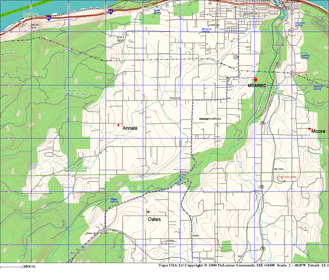
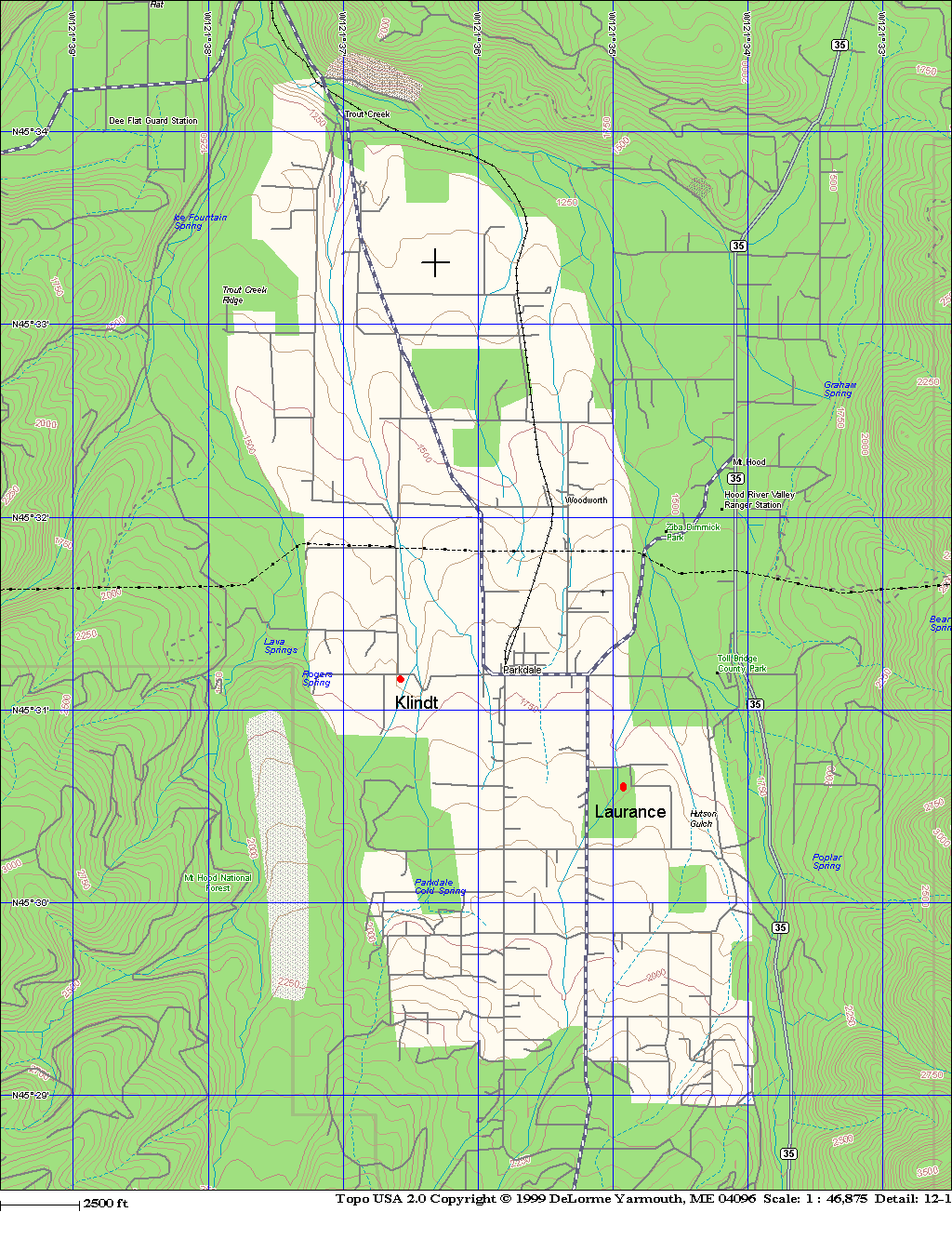
Table 1. Verification and validation data for 4km, gaussian smoothing, and least squares downscale techniques used for producing degree-day maps in Figs. 1-3 above. Click on station names for location map of grower-run stations.

									BUILD Model Results
Station	Station	Station	Actual	Elev	Elev	Est DD	Est DD	Est DD	Slope	Intercept	Corr.	Residual
Longitude	Latitude	Name	site DD	4km	500m	4km	500m GAUSS	500m Downscale	B1	B0	coeff.	Yi - Yhat
1. Stations included from the analysis (verification data)
121:35:00.00W	45:31:00.00N	PARO	2647	600	528	2632	2591	2657	-8.303	16793.34	-.93	-50
121:30:07.00W	45:38:52.00N	PNGO	2968	203	212	3123	2963	3189	-11.403	20237.14	-.94	-96
121:31:01.00W	45:41:00.00N	HOXO	3410	203	135	3123	3315	3274	-9.394	19639.10	-.81	71
121:37:55.00W	45:35:08.00N	DEFO	2748	376	279	2751	2706	2953	-9.060	18157.79	-.86	-62
121:12:05.00W	45:36:01.00N	T_Dalles	4265	182	69	4266	4335	4448	-21.385	29003.83	-.95	104
correlation: EST DD vs actual DD						0.970	0.998	0.973
2. Hood River stations excluded from the analysis (validation data)
121:34:37.51W	45:40:13.37N	Annala	3071	295	255	3065	3138	3098	-8.908	19211.18	-.81	-7
121:33:52.44W	45:38:34.73N	Oates	3111	384	227	2899	3025	3102	-10.203	19209.27	-.91	-14
121:31:01.16W	45:41:07.18N	MCAREC	3257	203	155	3123	3331	3249	-9.394	19639.10	-.81	71
121:29:31.02W	45:40:13.00N	Moore	2837	203	208	3123	3139	3224	-10.023	20207.59	-.84	13
121:31:10.18W	45:36:29.17N	Nakamura	3062	311	353	2725	2708	2926	-10.420	19214.75	-.92	-94
121:36:34.70W	45:31:06.31N	Klindt	2635	671	511	2490	2602	2685	-9.261	17388.52	-.92	-34
121:34:55.54W	45:30:39.41N	Laurance	2422	600	534	2632	2567	2650	-8.303	16793.34	-.93	-49
correlation: EST DD vs actual DD						0.673	0.764	0.810

References:
Fotheringham, A. S., C. Brunsdon, and M. Charlton. 2002. Geographically Weighted Regression – the analysis of spatially varying relationships. J. Wiley & Sons.269 pp.

On-line since April 5, 1996
This page last updated Mar 25, 2004
Contact Len Coop at coopl@bcc.orst.edu if you have any questions about this information.